Online Parameter Identification

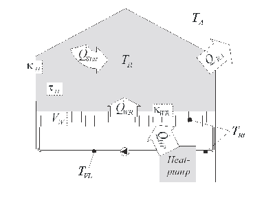
To solve the model predictive control problem, a dynamic linear model of the house is required. Preceding studies have shown that a model of second order is able to describe the most important dynamics.

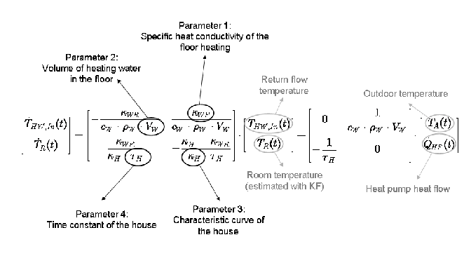
The model for the controller is based on simple thermodynamic laws, the resulting differential equation system can be written as a state space model:

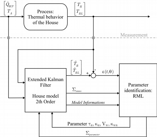
The required measurement data are the outdoor temperature, the on/off state of the heat pump, and the return flow temperature. If it is not measured, the room temperature is estimated with a Kalman filter by means of the linear model. The resulting equations contain four a priori unknown parameters; furthermore, since the parameters of the model differ from one house to another, an identification mechanism is indispensable.
Many approaches can be used to solve the system identification problem. For the specific case of this project (the second-order house model), parametric identification methods are used. The identification algorithm must satisfy the following conditions:

• Robustness in respect to disturbances such as measurement noise and modeling errors.
• Detection of the solar radiation and consideration of the mean gained energy in the model.
• Recursive implementation of the algorithm to permit the real-time identification of the parameters in an industrial heat-pump controller.
• The identified model must be able to anticipate reliably the house dynamics for the next day.

Three families of recursive parameter identification methods have been analyzed:

• Pseudo-Linear Regression Methods: They include the identification methods, whose model structures can be expressed as a linear regression and thus may be solved with the least squares method.
• Prediction Error Methods: This family focuses on the minimization of a cost function of the error between measured and estimated signals. Since generally there exists no analytic solution to the minimization problem, numerical search algorithms (such as the Gauss-Newton method) are used. An example is the recursive maximum likelihood method (RML).
• Bayesian Approach: These methods model the parameters as random variables. Starting from a priori density function of the parameter, the a posteriori density function is estimated at each time step based on the new measurements. The parameters are thus estimated evaluating the a posteriori density function. An example is the extended Kalman filter (EKF).

Results have shown that recursive and offline least-squares methods are inadequate for the task of parameter identification, since the estimated parameters are biased. Thus the identified model cannot reproduce the house dynamics and is often unstable.
Better results can be obtained with the family of the prediction error methods, because these are not restricted to the ARX model structures. In particular, the maximum likelihood method applied to a Kalman Filter or an Output Error Structure as a predictor has been analyzed and has delivered good approximations of the parameters.
The Extended Kalman Filter also has proved to be a useful tool for the parameter identification.